Quantifying differential rhythmicity between conditions
Source:vignettes/differential-rhythmicity.Rmd
differential-rhythmicity.RmdIntroduction
Here we show how to use limorhyde2 to quantify rhythmicity and differential rhythmicity in data from multiple conditions. The data are based on liver samples from wild-type and Rev-erb\(\alpha/\beta\) double-knockout mice (Cho et al. 2012 and GSE34018).
Load packages
library('data.table')
library('ggplot2')
library('limorhyde2')
library('qs')

# doParallel::registerDoParallel() # register a parallel backend to minimize runtime
theme_set(theme_bw())
Load the data
The expression data are in a matrix with one row per gene and one column per sample. The metadata are in a table with one row per sample. To save time and space, the expression data include only a subset of genes.
y = qread(system.file('extdata', 'GSE34018_data.qs', package = 'limorhyde2'))
y[1:5, 1:5]
#>       GSM840516 GSM840517 GSM840518 GSM840519 GSM840520
#> 12686 11.962830 11.923338 11.098814 10.958933  9.256413
#> 13170  8.989743  9.132606 12.381036 12.441759 14.766070
#> 26897 11.515292 11.625519 10.579969 10.601969 11.096489
#> 11287  7.985859  7.930935  7.674688  7.899531  7.768563
#> 11731  8.481372  8.114623  8.058194  8.144267  8.152959

metadata = qread(system.file('extdata', 'GSE34018_metadata.qs', package = 'limorhyde2'))
metadata
#>        sample      cond time
#>  1: GSM840516 wild-type    0
#>  2: GSM840517 wild-type    0
#>  3: GSM840518 wild-type    4
#>  4: GSM840519 wild-type    4
#>  5: GSM840520 wild-type    8
#>  6: GSM840521 wild-type    8
#>  7: GSM840522 wild-type   12
#>  8: GSM840523 wild-type   12
#>  9: GSM840524 wild-type   16
#> 10: GSM840525 wild-type   16
#> 11: GSM840526 wild-type   20
#> 12: GSM840527 wild-type   20
#> 13: GSM840504  knockout    0
#> 14: GSM840505  knockout    0
#> 15: GSM840506  knockout    4
#> 16: GSM840507  knockout    4
#> 17: GSM840508  knockout    8
#> 18: GSM840509  knockout    8
#> 19: GSM840510  knockout   12
#> 20: GSM840511  knockout   12
#> 21: GSM840512  knockout   16
#> 22: GSM840513  knockout   16
#> 23: GSM840514  knockout   20
#> 24: GSM840515  knockout   20
#>        sample      cond time
Fit linear models and compute posterior fits
Because the samples were acquired at relatively low temporal resolution (every 4 h), we use three knots instead of the default four, which reduces the flexibility of the spline curves. We specify condColname so getModelFit() knows to fit a differential rhythmicity model.
fit = getModelFit(y, metadata, nKnots = 3L, condColname = 'cond')
fit = getPosteriorFit(fit)
#>  - Computing 100 x 109 likelihood matrix.
#>  - Likelihood calculations took 0.09 seconds.
#>  - Fitting model with 109 mixture components.
#>  - Model fitting took 0.03 seconds.
#>  - Computing posterior matrices.
#>  - Computation allocated took 0.02 seconds.
Get rhythmic statistics
Next, we use the posterior fits to compute rhythmic statistics for each gene in each condition.
rhyStats = getRhythmStats(fit)
print(rhyStats, nrows = 10L)
#>           cond   feature peak_phase peak_value trough_phase trough_value
#>   1: wild-type     12686  23.583282  11.844107   10.4736761     8.785513
#>   2: wild-type     13170   9.444423  15.019936   22.2707495     9.113807
#>   3: wild-type     26897  18.166330  12.367458    4.7795034    10.697741
#>   4: wild-type     11287  21.613506   7.921370    7.5466856     7.778185
#>   5: wild-type     11731  16.271138   8.251227    4.8812985     8.207653
#>  ---
#> 196:  knockout    382038  17.994402   8.122326    0.4356467     8.030396
#> 197:  knockout    404323   6.101673   8.070874   23.1863197     8.063530
#> 198:  knockout    435684  10.576267   8.292289   19.1186125     8.287769
#> 199:  knockout    622408   6.101719   7.927632   23.6722205     7.902385
#> 200:  knockout 110599566  21.559365   8.922764   12.6101340     8.909615
#>      peak_trough_amp     rms_amp mean_value
#>   1:     3.058593622 1.073445705  10.368427
#>   2:     5.906128877 2.078735725  12.018767
#>   3:     1.669716330 0.594546001  11.675870
#>   4:     0.143185025 0.049291689   7.854743
#>   5:     0.043574326 0.015641890   8.233332
#>  ---
#> 196:     0.091930147 0.027487564   8.072759
#> 197:     0.007343261 0.002194299   8.067516
#> 198:     0.004520197 0.001443692   8.290186
#> 199:     0.025246670 0.007586063   7.916088
#> 200:     0.013148403 0.004548861   8.917391
Get differentially rhythmic statistics
We can now calculate the rhythmic differences for each gene between any two conditions, here between wild-type and knockout.
diffRhyStats = getDiffRhythmStats(fit, rhyStats)
print(diffRhyStats, nrows = 10L)
#>        feature     cond1    cond2 diff_mean_value diff_peak_trough_amp
#>   1:    101476 wild-type knockout     0.385079194         -0.119024736
#>   2:    104662 wild-type knockout    -0.088926109         -0.120641471
#>   3:    107652 wild-type knockout     0.030761445         -0.343503780
#>   4:    109359 wild-type knockout     0.009406463         -0.039640031
#>   5: 110599566 wild-type knockout    -0.006050343         -0.057446071
#>  ---
#>  96:     76629 wild-type knockout    -0.045727952         -0.025321758
#>  97:     78174 wild-type knockout     0.003833334         -0.002883578
#>  98:     80782 wild-type knockout     0.019076587         -0.026706196
#>  99:     93671 wild-type knockout    -0.122202398          0.318458377
#> 100:     97064 wild-type knockout    -0.066047812         -0.057648476
#>      diff_rms_amp diff_peak_phase diff_trough_phase rms_diff_rhy
#>   1: -0.050009025      -1.5431221        -3.6419347  0.231750686
#>   2: -0.048870179       7.5438911         5.1482949  0.201688499
#>   3: -0.115274715      -2.3486873        -4.2596862  0.390392048
#>   4: -0.014145087      -0.7842197        -3.2539909  0.045821389
#>   5: -0.019823612       8.0133286         7.9850954  0.079889026
#>  ---
#>  96: -0.009408998       6.4503647         8.6171045  0.041815280
#>  97: -0.001211714       1.6270477        -2.0338405  0.004473018
#>  98: -0.009274696       0.1900240        -0.4066909  0.028202979
#>  99:  0.102493077      -3.5169301        11.3633377  1.044134449
#> 100: -0.020596285      -2.0915970        -7.9439872  0.068376386
We can examine the distributions of the statistics in various ways, such as ranking genes by difference in peak-to-trough amplitude (no p-values necessary) or plotting difference in peak-to-trough amplitude vs. difference in mean expression.
print(diffRhyStats[order(diff_peak_trough_amp)], nrows = 10L)
#>      feature     cond1    cond2 diff_mean_value diff_peak_trough_amp
#>   1:   13170 wild-type knockout     1.200806055         -3.533865155
#>   2:   12686 wild-type knockout    -0.414207921         -2.406530463
#>   3:   26897 wild-type knockout    -2.388261031         -1.034124834
#>   4:   20211 wild-type knockout    -1.131052863         -0.699250756
#>   5:   12977 wild-type knockout    -0.027363903         -0.473937425
#>  ---
#>  96:  329910 wild-type knockout    -0.084197747          0.003591791
#>  97:   20497 wild-type knockout     0.023894611          0.004206791
#>  98:   58229 wild-type knockout    -0.005650829          0.004711548
#>  99:   18378 wild-type knockout    -0.059531404          0.088706917
#> 100:   93671 wild-type knockout    -0.122202398          0.318458377
#>       diff_rms_amp diff_peak_phase diff_trough_phase rms_diff_rhy
#>   1: -1.2402582569      -0.9555117        -0.5424612  3.802135940
#>   2: -0.8550873280      -4.9265939        -1.1261574  2.828991912
#>   3: -0.3915656446       0.7545927         6.2343634  1.479902146
#>   4: -0.2563897925      -2.7175892       -10.1197405  1.241164124
#>   5: -0.1682833503      -1.3111235        -4.7103687  0.521668016
#>  ---
#>  96:  0.0031446455       9.0552937         9.5536510  0.197597118
#>  97:  0.0008941407       8.1356528         8.3626192  0.018547619
#>  98:  0.0013749504      10.9831840        -3.2542325  0.007650559
#>  99:  0.0237101323       9.3201219         8.6090161  0.256049333
#> 100:  0.1024930767      -3.5169301        11.3633377  1.044134449

ggplot(diffRhyStats) +
  geom_point(aes(x = diff_mean_value, y = diff_peak_trough_amp), alpha = 0.2) +
  labs(x = 'Difference in mean expression (norm.)',
       y = 'Difference in peak-to-trough amplitude (norm.)')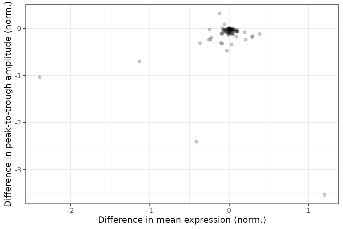
Get observed and fitted time-courses
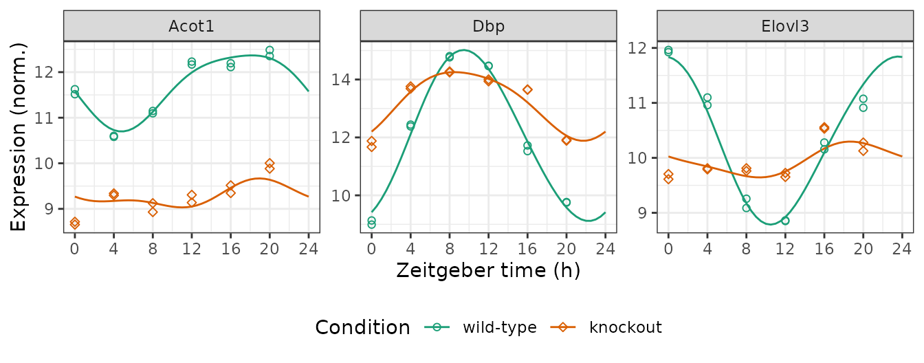
We can compute the expected measurements for one or more genes at one or more time-points in each condition, which correspond to the fitted curves. Here we plot the posterior fits and observed expression for three genes (converting from gene id to gene symbol).
genes = data.table(id = c('13170', '12686', '26897'),
                   symbol = c('Dbp', 'Elovl3', 'Acot1'))

measFit = getExpectedMeas(fit, times = seq(0, 24, 0.5), features = genes$id)
measFit[genes, symbol := i.symbol, on = .(feature = id)]
print(measFit, nrows = 10L)
#>      time      cond feature     value symbol
#>   1:    0 wild-type   13170  9.416439    Dbp
#>   2:    0 wild-type   12686 11.835367 Elovl3
#>   3:    0 wild-type   26897 11.575952  Acot1
#>   4:    0  knockout   13170 12.200770    Dbp
#>   5:    0  knockout   12686 10.025091 Elovl3
#>  ---
#> 290:   24 wild-type   12686 11.835367 Elovl3
#> 291:   24 wild-type   26897 11.575952  Acot1
#> 292:   24  knockout   13170 12.200770    Dbp
#> 293:   24  knockout   12686 10.025091 Elovl3
#> 294:   24  knockout   26897  9.268390  Acot1
Next we combine the observed expression data and metadata. The curves show how limorhyde2 is able to fit non-sinusoidal rhythms.
measObs = mergeMeasMeta(y, metadata, features = genes$id)
measObs[genes, symbol := i.symbol, on = .(feature = id)]
print(measObs, nrows = 10L)
#>        sample      cond time feature      meas symbol
#>  1: GSM840504  knockout    0   13170 11.669138    Dbp
#>  2: GSM840504  knockout    0   12686  9.705361 Elovl3
#>  3: GSM840504  knockout    0   26897  8.654624  Acot1
#>  4: GSM840505  knockout    0   13170 11.877697    Dbp
#>  5: GSM840505  knockout    0   12686  9.611530 Elovl3
#> ---
#> 68: GSM840526 wild-type   20   12686 10.911935 Elovl3
#> 69: GSM840526 wild-type   20   26897 12.486105  Acot1
#> 70: GSM840527 wild-type   20   13170  9.749365    Dbp
#> 71: GSM840527 wild-type   20   12686 11.075636 Elovl3
#> 72: GSM840527 wild-type   20   26897 12.352601  Acot1

ggplot() +
  facet_wrap(vars(symbol), scales = 'free_y', nrow = 1) +
  geom_line(aes(x = time, y = value, color = cond), data = measFit) +
  geom_point(aes(x = time %% 24, y = meas, color = cond, shape = cond),
             size = 1.5, data = measObs) +
  labs(x = 'Zeitgeber time (h)', y = 'Expression (norm.)',
       color = 'Condition', shape = 'Condition') +
  scale_x_continuous(breaks = seq(0, 24, 4)) +
  scale_color_brewer(palette = 'Dark2') +
  scale_shape_manual(values = c(21, 23)) +
  theme(legend.position = 'bottom')